
On this page:
3.1.2 Limitation of physical measurements
Represent uncertainty in a data point on a graph using error bars.
Determine the uncertainties in the gradient and intercept of a straight-line graph.
Individual points on the graph may or may not have associated error bars.
Drawing graphs and lines of best fit
A single measurement only ever gives us one number, and one number on its own can be misleading — it might be a fluke, or it might have been affected by an error we haven’t spotted. When we take a whole series of readings and plot them as a graph, the pattern that emerges is far more convincing than any individual point, and it lets us pull out genuine physical quantities, such as a spring constant or the acceleration due to gravity, from the shape of the line rather than from a single reading.
Before any of that is possible the graph itself has to be drawn well. A few habits make the difference between a graph that is genuinely useful and one that just looks like a graph:
- Choose a scale that spreads the data across as much of the graph as possible – a tiny cluster of points squeezed into one corner throws away precision.
- Avoid awkward scales such as multiples of 3 or 7, which make plotting and reading off values needlessly difficult.
- Label both axes clearly with the quantity and its unit, for example “extension / m”.
- Plot each point precisely as a small, sharp cross or an encircled dot, so that its centre is unambiguous.
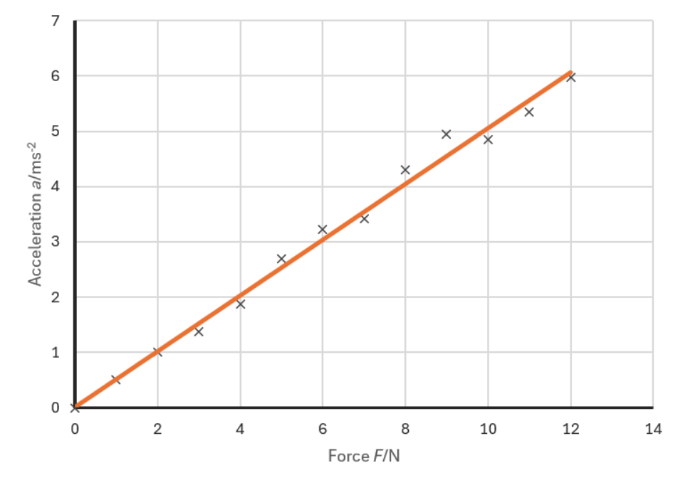
Once the points are plotted we draw a line of best fit – a single straight line (or, occasionally, a smooth curve) positioned so that it passes as close as possible to all of the points, with roughly as many points scattered above the line as below it. It will not usually pass exactly through every point, and that is fine: the scatter is a reflection of the random error in the measurements, not a mistake in the drawing.
Common exam mistake
Don’t join the points dot-to-dot — a zig-zag line through every point treats each reading as if it were perfect, when in reality every point carries some random error. A single smooth line of best fit represents your best estimate of the true underlying trend. In the same way, never force the line through the origin just because you expect the relationship to pass through zero — only draw it there if the data genuinely supports it.
Once we have this single line, it becomes the tool we use for everything else on this page: reading off the gradient, finding the intercept, and working out how much we can trust both of those values.
Error bars and the worst acceptable line
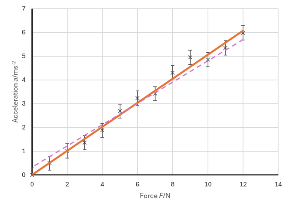
We have already seen that every measurement carries an uncertainty. On a graph, we show this uncertainty for each point using an error bar – a short line extending above and below the point (or left and right, if the uncertainty in the x-value is significant) by an amount equal to the absolute uncertainty in that reading. The error bar effectively marks out a small range within which the true value of that point is expected to lie.
Individual points don’t always need error bars – if the uncertainty is too small to show clearly at the scale of the graph, or if only one axis has a significant uncertainty, then bars are only drawn where they matter. Where they are shown, though, they give us a powerful tool: a way of turning a scatter of individual uncertainties into a single, useful uncertainty in the gradient of the whole line.
This is done by drawing a second line, the worst acceptable line – the most steeply or shallowly sloped straight line that still passes through every error bar. Rather than being shifted bodily up or down from the line of best fit, it should pivot through a sensible point near the middle of the data, since it represents a genuinely different but still plausible interpretation of the same data set, not just a parallel copy of the best-fit line.
Common exam mistake
A worst line that is simply the best-fit line shifted up or down, still with the same gradient, tells us nothing new — it has to be rotated to a different gradient while still staying within every error bar. It’s also easy to forget that the worst line must remain a straight line and a reasonable fit — a line that only touches one error bar while ignoring the rest isn’t acceptable, however extreme a gradient it lets you claim.
Finding the gradient and the intercept
With the line of best fit drawn, we can extract two useful numbers from it: the gradient and the intercept. Both are read directly from points on the line, not from individual data points, which may not lie exactly on it.
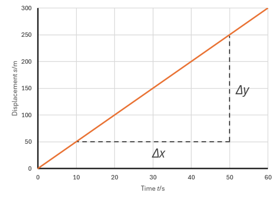
To find the gradient, draw as large a triangle as possible under the line – ideally spanning at least half its length – and read off the change in y and the change in x from its two shorter sides:
The larger the triangle, the more precisely the gradient can be read, since any small error in reading a coordinate matters far less when spread over a bigger triangle. The gradient always carries a unit too – whatever the unit of y is, divided by the unit of x – so a gradient is rarely just a bare number.
The intercept is the value of y where the line crosses the y-axis, at $x=0$. If the axes don’t extend back as far as $x=0$, extend the line of best fit backwards with a dashed extrapolation line until it does, or calculate it algebraically using $y=mx+c$ with the gradient and a single point taken from the line.
Once we have drawn the worst acceptable line as well, finding the uncertainty in the gradient and intercept is simply a case of comparing the two lines. The uncertainty in the gradient is the difference between the best-fit gradient and the worst-fit gradient, and the same idea applies to the intercept:
This can then be expressed as a percentage uncertainty in the usual way, and, since a physical quantity is very often calculated directly from the gradient, that percentage uncertainty carries straight through into the final result.
Worth remembering
Choosing what to plot is itself part of the skill. Many relationships in this course aren’t naturally straight lines — but they can often be rearranged into the form $y=mx+c$ by plotting a different combination of variables, turning a curve into a straight line whose gradient or intercept is exactly the physical constant we’re after. We’ll see this in the worked example below.
Common exam mistake
Don’t forget the units on a gradient — stating a gradient as simply “4.00” instead of “4.00 s2 m−1” loses marks even if the number itself is correct. Also make sure the triangle used to calculate the gradient is large enough; a triangle only a centimetre or two wide magnifies any small reading error into a large error in the final gradient.
Worked example
A student investigates how the period of a simple pendulum depends on its length by measuring the time period, T, for a range of lengths, L. Since $T=2\pi\sqrt{\frac{L}{g}}$, a graph of T against L would be a curve, so instead the student plots $T^2$ against L, giving a straight line through the origin:
Figure 4 shows the student’s results, with a line of best fit and a worst acceptable line drawn through the error bars.
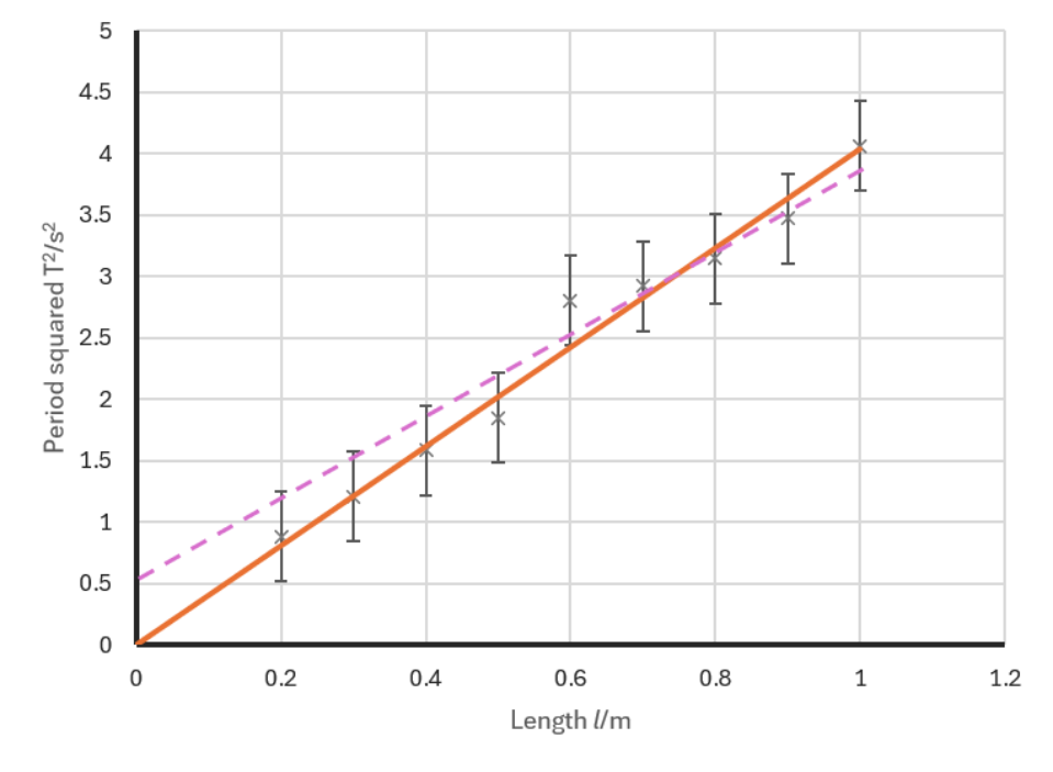
- Use Figure 4 to determine the gradient of the line of best fit and its uncertainty.
- Use the gradient found in part a) to calculate a value for g.
- State the absolute uncertainty in g, and comment on the result.
Drawing as large a triangle as possible under the line of best fit gives a gradient of $\quantity{4.00}{s^2\,m^{-1}}$. Doing the same for the worst acceptable line gives a gradient of $\quantity{3.70}{s^2\,m^{-1}}$, so the uncertainty in the gradient is:
As a percentage, this is $\frac{0.30}{4.00}\times100=7.5\%$.
Comparing $T^2=\left(\frac{4\pi^2}{g}\right)L$ with the gradient found above, $g=\frac{4\pi^2}{\mathrm{gradient}}$:
Notice that, because the graph passes through the origin, there’s no intercept to find here – not every graph needs one.
Since $g$ is inversely proportional to the gradient, the percentage uncertainty carries straight across: the percentage uncertainty in $g$ is also 7.5%, giving an absolute uncertainty of:
So the student’s result is $g=(9.9\pm0.7)\ \mathrm{m\,s^{-2}}$. This comfortably includes the accepted value of $\quantity{9.81}{m\,s^{-2}}$, so despite a fairly large percentage uncertainty the experiment has worked well — a result worth remembering when a large uncertainty makes an experiment feel like a failure, when in fact it has correctly captured the true value within its range.